Visual and analytic solution comparison
The idea here is to compare the various analytic functions with approximate solutions, to verify that the analytic implementation is correct. Ideally, we want to see two things:
- As the number of approximation points increases, the error should go down and tend towards zero.
- With a sufficient number of approximation points, the analytic and approximate solutions should appear visually identical.
# imports
%matplotlib inline
from bayesian_quadrature import BQ, bq_c, gauss_c, util
from gp import GaussianKernel

# set loglevel to debug
import logging
logger = logging.getLogger("bayesian_quadrature")
logger.setLevel("DEBUG")
# seed the numpy random generator, so we always get the same randomness
np.random.seed(8728)
# parameters
options = {
    'n_candidate': 10,
    'x_mean': 0.0,
    'x_var': 10.0,
    'candidate_thresh': 0.5,
    'kernel': GaussianKernel,
    'optim_method': 'L-BFGS-B'
}

# different number of approximation points to try, to see if the
# approximation converges, and the range over which we will compute
# the approximation points
N = np.logspace(np.log10(30), np.log10(500), 100)
xmin, xmax = -10, 10
Here we define some helper functions to plot the error/visual comparisons, and to print information about the worst error and approximate/analytic solution values.
def plot_0d(calc, approx):
    fig, ax = plt.subplots()
    ax.plot(N, np.abs(calc - approx), lw=2, color='r')
    ax.set_title("Error")
    ax.set_xlabel("# approximation points")
    ax.set_xlim(N.min(), N.max())
    util.set_scientific(ax, -5, 4)
def print_0d(calc, approx):
    err = np.abs(calc - approx[-1])
    print "error : %s" % err
    print "approx: %s" % approx[-1]
    print "calc  : %s" % calc
def plot_1d(calc, approx):
    fig, (ax1, ax2) = plt.subplots(1, 2)

    ax1.plot(N, np.abs(calc[:, None] - approx).sum(axis=0), lw=2, color='r')
    ax1.set_title("Error")
    ax1.set_xlabel("# approximation points")
    ax1.set_xlim(N.min(), N.max())
    util.set_scientific(ax1, -5, 4)

    ax2.plot(approx[:, -1], lw=2, label="approx")
    ax2.plot(calc, '--', lw=2, label="calc")
    ax2.set_title("Comparison")
    ax2.legend(loc=0)
    util.set_scientific(ax2, -5, 4)

    fig.set_figwidth(8)
    plt.tight_layout()
def print_1d(calc, approx):
    maxerr = np.abs(calc - approx[..., -1]).max()
    approx_sum, calc_sum = approx[..., -1].sum(), calc.sum()
    print "max error  : %s" % maxerr
    print "sum(approx): %s" % approx_sum
    print "sum(calc)  : %s" % calc_sum
def plot_2d(calc, approx):
    fig, (ax1, ax2, ax3, ax4) = plt.subplots(1, 4)

    ax1.plot(N, np.abs(calc[:, :, None] - approx).sum(axis=0).sum(axis=0), lw=2, color='r')
    ax1.set_title("Error")
    ax1.set_xlabel("# approximation points")
    ax1.set_xlim(N.min(), N.max())
    util.set_scientific(ax1, -5, 4)

    vmax = max(approx[:, :, -1].max(), calc.max())

    ax2.imshow(approx[:, :, -1], cmap='gray', interpolation='nearest', vmin=0, vmax=vmax)
    ax2.set_title("Approximation")

    ax3.imshow(calc, cmap='gray', interpolation='nearest', vmin=0, vmax=vmax)
    ax3.set_title("Calculated")

    i = 0
    ax4.plot(approx[i, :, -1], lw=2, label='approx')
    ax4.plot(calc[i], '--', lw=2, label='calc')
    ax4.set_title("Comparison at index %d" % i)
    ax4.legend(loc=0)
    util.set_scientific(ax4, -5, 4)

    fig.set_figwidth(14)
    plt.tight_layout()
Now we create the Bayesian Quadrature object that we’ll be testing against.
# choose points and evaluate them under a standard normal distribution
x = np.linspace(-5, 5, 9)
f_y = lambda x: scipy.stats.norm.pdf(x, 0, 1)
y = f_y(x)
# create the bayesian quadrature object
bq = BQ(x, y, **options)
bq.init(
params_tl=(15, 2, 0.),
params_l=(0.2, 1.3, 0.))
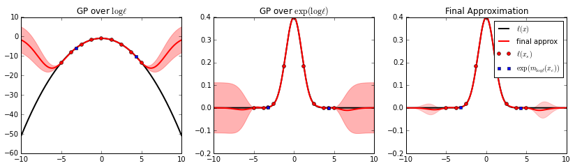
# plot the BQ approximation
fig, axes = bq.plot(f_l=f_y, xmin=xmin, xmax=xmax)
DEBUG:bayesian_quadrature:Choosing candidate points
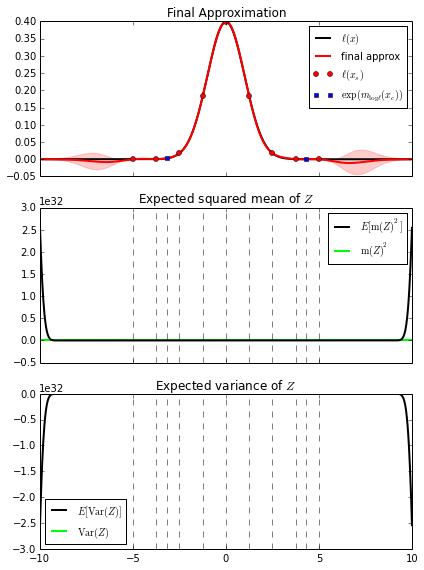
fig, (ax1, ax2, ax3) = plt.subplots(3, 1, sharex=True)
xmin, xmax = -10, 10
bq.plot_l(ax1, f_l=f_y, xmin=xmin, xmax=xmax)
bq.plot_expected_squared_mean(ax2, xmin=xmin, xmax=xmax)
bq.plot_expected_variance(ax3, xmin=xmin, xmax=xmax)
fig.set_figheight(8)
plt.tight_layout()
x_l = np.array(bq.gp_l.x[None], order='F')
h_l = bq.gp_l.K.h
w_l = np.array([bq.gp_l.K.w], order='F')

x_tl = np.array(bq.gp_log_l.x[None], order='F')
h_tl = bq.gp_log_l.K.h
w_tl = np.array([bq.gp_log_l.K.w], order='F')

xm = bq.options['x_mean']
xC = bq.options['x_cov']
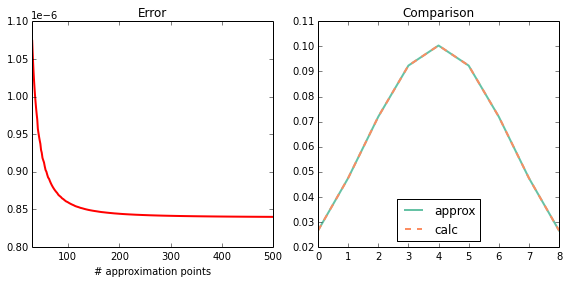
int_K
Test \(\int K(x^\prime, x) \mathcal{N}(x^\prime | \mu, \Sigma)\ \mathrm{d}x^\prime\)
calc = np.empty(bq.nsc, order='F')
gauss_c.int_K(calc, x_l, h_l, w_l, xm, xC)

approx = np.empty((bq.nsc, N.size), order='F')
for i, n in enumerate(N):
    xo = np.linspace(xmin, xmax, n)
    Kxxo = np.array(bq.gp_l.Kxxo(xo), order='F')
    gauss_c.approx_int_K(
        approx[:, i],
        np.array(xo[None], order='F'),
        Kxxo, xm, xC)
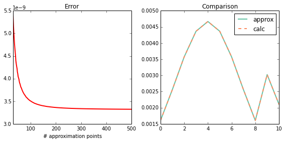
plot_1d(calc, approx)
print_1d(calc, approx)
max error  : 1.55678221442e-09
sum(approx): 0.0339891854186
sum(calc)  : 0.033989188741
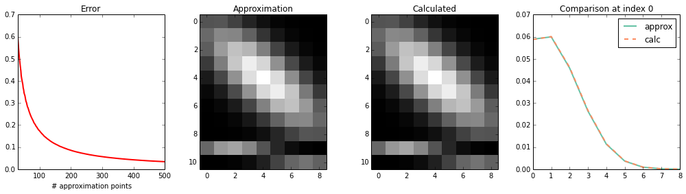
int_K1_K2
Test \(\int K_1(x_1, x^\prime) K_2(x^\prime, x_2) \mathcal{N}(x^\prime | \mu, \Sigma)\ \mathrm{d}x^\prime\)
calc = np.empty((bq.nsc, bq.ns), order='F')
gauss_c.int_K1_K2(calc, x_l, x_tl, h_l, w_l, h_tl, w_tl, xm, xC)

approx = np.empty((bq.nsc, bq.ns, N.size), order='F')
for i, n in enumerate(N):
    xo = np.linspace(xmin, xmax, n)
    K1xxo = np.array(bq.gp_l.Kxxo(xo), order='F')
    K2xxo = np.array(bq.gp_log_l.Kxxo(xo), order='F')
    gauss_c.approx_int_K1_K2(
        approx[:, :, i],
        np.array(xo[None], order='F'),
        K1xxo, K2xxo, xm, xC)
plot_2d(calc, approx)
print_1d(calc, approx)
max error  : 0.000933347326451
sum(approx): 5.55089408134
sum(calc)  : 5.55090592396
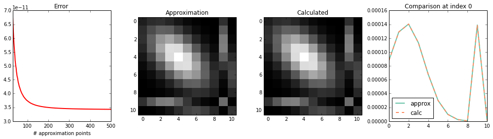
int_int_K1_K2_K1
Test \(\int \int K_1(x, x_1^\prime) K_2(x_1^\prime, x_2^\prime) K_1(x_2^\prime, x) \mathcal{N}(x_1^\prime | \mu, \Sigma) \mathcal{N}(x_2^\prime | \mu, \Sigma)\ \mathrm{d}x_1^\prime\ \mathrm{d}x_2^\prime\)
calc = np.empty((bq.nsc, bq.nsc), order='F')
gauss_c.int_int_K1_K2_K1(calc, x_l, h_l, w_l, h_tl, w_tl, xm, xC)

approx = np.empty((bq.nsc, bq.nsc, N.size), order='F')
for i, n in enumerate(N):
    xo = np.linspace(xmin, xmax, n)
    K1xxo = np.array(bq.gp_l.Kxxo(xo), order='F')
    K2xoxo = np.array(bq.gp_log_l.Kxoxo(xo), order='F')
    gauss_c.approx_int_int_K1_K2_K1(
        approx[:, :, i],
        np.array(xo[None], order='F'),
        K1xxo, K2xoxo, xm, xC)
plot_2d(calc, approx)
print_1d(calc, approx)
max error  : 7.56401320431e-12
sum(approx): 0.0230979040561
sum(calc)  : 0.0230979040904
int_int_K1_K2
Test \(\int \int K_1(x_2^\prime, x_1^\prime) K_2(x_1^\prime, x) \mathcal{N}(x_1^\prime | \mu, \Sigma) \mathcal{N}(x_2^\prime | \mu, \Sigma)\ \mathrm{d}x_1^\prime\ \mathrm{d}x_2^\prime\)
calc = np.empty(bq.ns, order='F')
gauss_c.int_int_K1_K2(calc, x_tl, h_l, w_l, h_tl, w_tl, xm, xC)

approx = np.empty((bq.ns, N.size), order='F')
for i, n in enumerate(N):
    xo = np.linspace(xmin, xmax, n)
    K1xoxo = np.array(bq.gp_l.Kxoxo(xo), order='F')
    K2xxo = np.array(bq.gp_log_l.Kxxo(xo), order='F')
    gauss_c.approx_int_int_K1_K2(
        approx[:, i],
        np.array(xo[None], order='F'),
        K1xoxo, K2xxo, xm, xC)
plot_1d(calc, approx)
print_1d(calc, approx)
max error  : 2.90292116595e-07
sum(approx): 0.576959029431
sum(calc)  : 0.576959869272
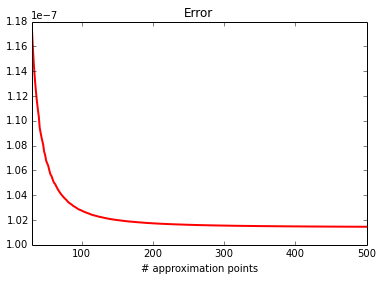
int_int_K
Test \(\int \int K(x_1^\prime, x_2^\prime) \mathcal{N}(x_1^\prime | \mu, \Sigma) \mathcal{N}(x_2^\prime | \mu, \Sigma)\ \mathrm{d}x_1^\prime\ \mathrm{d}x_2^\prime\)
calc = gauss_c.int_int_K(1, h_l, w_l, xm, xC)

approx = np.empty(N.size, order='F')
for i, n in enumerate(N):
    xo = np.linspace(xmin, xmax, n)
    Kxoxo = np.array(bq.gp_l.Kxoxo(xo), order='F')
    approx[i] = gauss_c.approx_int_int_K(
        np.array(xo[None], order='F'), Kxoxo, xm, xC)
plot_0d(calc, approx)
print_0d(calc, approx)
error : 1.01454767464e-07
approx: 0.00342631605819
calc  : 0.00342641751296
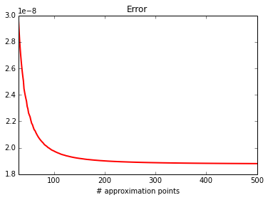
Mean of Z
Test \(E[Z]\).
calc = bq._exact_Z_mean()
approx = np.empty(N.size)
for i, n in enumerate(N):
    xo = np.linspace(xmin, xmax, n)
    approx[i] = bq._approx_Z_mean(xo)
plot_0d(calc, approx)
print_0d(calc, approx)
error : 1.8803056015e-08
approx: 0.119771024599
calc  : 0.119771005796
Variance of Z
Test \(\mathrm{Var}(Z)\).
calc = bq._exact_Z_var()
approx = np.empty(N.size)
for i, n in enumerate(N):
    xo = np.linspace(xmin, xmax, n)
    approx[i] = bq._approx_Z_var(xo)
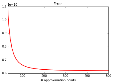
plot_0d(calc, approx)
print_0d(calc, approx)
error : 6.18632061484e-11
approx: 5.97977452085e-07
calc  : 5.98039315292e-07