Gaussian Kernel Example

# load matplotlib
%matplotlib inline

# imports
import numpy as np
import scipy.stats

# import the bayesian quadrature object
from bayesian_quadrature import BQ
from gp import GaussianKernel

# seed the numpy random generator, so we always get the same randomness
np.random.seed(8706)

First, we need to define various parameters:

options = {
    'n_candidate': 5,
    'x_mean': 0.0,
    'x_var': 10.0,
    'candidate_thresh': 0.5,
    'kernel': GaussianKernel,
    'optim_method': 'L-BFGS-B'
}

Now, sample some random \(x\) points and compute the \(y\) points from a standard normal distribution.

x = np.array([-1.75, -1, 1.25])
f_y = lambda x: scipy.stats.norm.pdf(x, 0, 1)
y = f_y(x)

Create the bayesian quadrature object, and fit its parameters.

bq = BQ(x, y, **options)
bq.init(params_tl=(15, 2, 0), params_l=(0.2, 1.3, 0))
bq.fit_hypers(['h', 'w'])

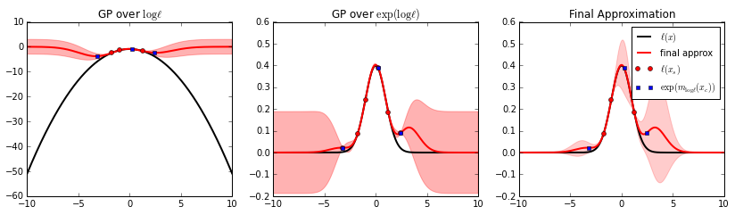
Plot the result.

fig, axes = bq.plot(f_y, xmin=-10, xmax=10)

Print out the mean and variance of the integral, \(Z\):

print "E[Z] = %f" % bq.Z_mean()
print "V(Z) = %f" % bq.Z_var()

E[Z] = 0.141767
V(Z) = 0.000737

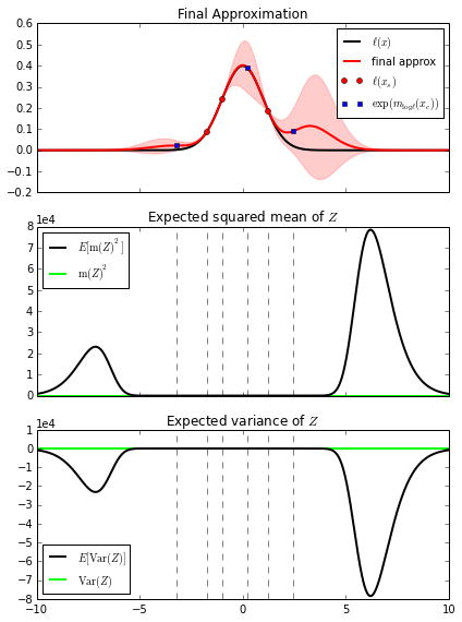
Compute the expected variance given a potential new observation, and then plot the curve of the expected variances, along with the final approximation.

fig, (ax1, ax2, ax3) = plt.subplots(3, 1, sharex=True)
xmin, xmax = -10, 10
bq.plot_l(ax1, f_l=f_y, xmin=xmin, xmax=xmax)
bq.plot_expected_squared_mean(ax2, xmin=xmin, xmax=xmax)
bq.plot_expected_variance(ax3, xmin=xmin, xmax=xmax)
fig.set_figheight(8)
plt.tight_layout()