Active Sampling Example

# load matplotlib
%matplotlib inline

# imports
import numpy as np
import scipy.stats
import scipy.optimize as optim

# import the bayesian quadrature object
from bayesian_quadrature import BQ
from gp import GaussianKernel

# seed the numpy random generator, so we always get the same randomness
np.random.seed(8706)

First, we need to define various parameters:

options = {
    'n_candidate': 10,
    'x_mean': 0.0,
    'x_var': 10.0,
    'candidate_thresh': 0.5,
    'kernel': GaussianKernel,
    'optim_method': 'L-BFGS-B'
}

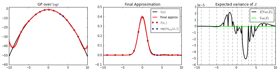
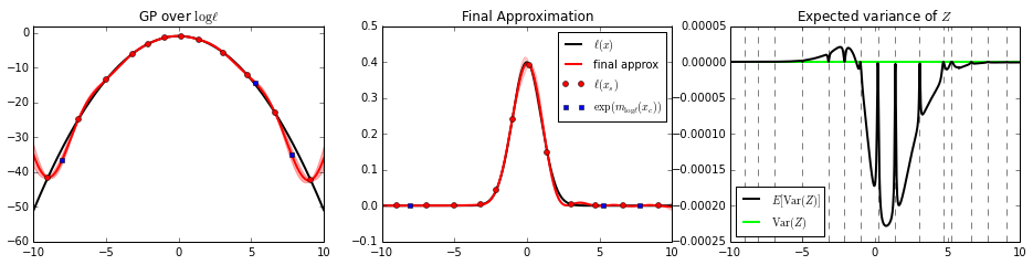
def plot(bq):
    fig, axes = plt.subplots(1, 3)
    xmin, xmax = -10, 10

    bq.plot_gp_log_l(axes[0], f_l=f_y, xmin=xmin, xmax=xmax)
    axes[0].set_ylim(-60, 2)

    bq.plot_l(axes[1], f_l=f_y, xmin=xmin, xmax=xmax)
    axes[1].set_ylim(-0.1, 0.5)

    bq.plot_expected_variance(axes[2], xmin=xmin, xmax=xmax)

    fig.set_figwidth(16)
    fig.set_figheight(3.5)

Now, sample some random \(x\) points and compute the \(y\) points from a standard normal distribution.

x = np.random.uniform(-5, -5, 1)
f_y = lambda x: scipy.stats.norm.pdf(x, 0, 1)
y = f_y(x)

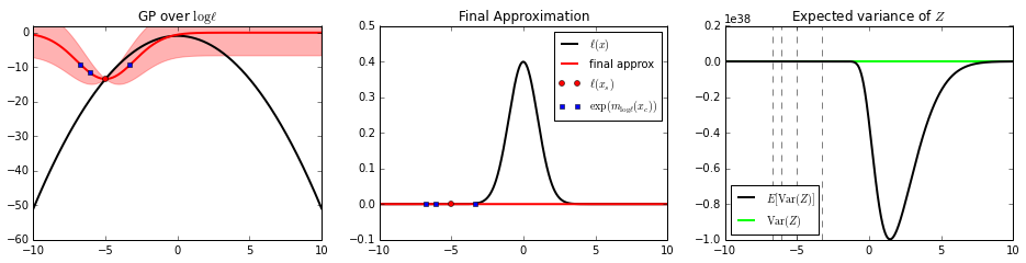
Create the bayesian quadrature object, and fit its parameters.

bq = BQ(x, y, **options)
bq.init(params_tl=(15, 2, 0), params_l=(0.2, 1.3, 0))
plot(bq)

def add(bq):
    params = ['h', 'w']

    x_a = np.sort(np.random.uniform(-10, 10, 20))
    x = bq.choose_next(x_a, n=100, params=params)
    print "x = %s" % x

    mean = bq.Z_mean()
    var = bq.Z_var()
    print "E[Z] = %s" % mean
    print "V(Z) = %s" % var

    conf = 1.96 * np.sqrt(var)
    lower = mean - conf
    upper = mean + conf
    print "Z = %.4f [%.4f, %.4f]" % (mean, lower, upper)

    bq.add_observation(x, f_y(x))
    bq.fit_hypers(params)
    plot(bq)

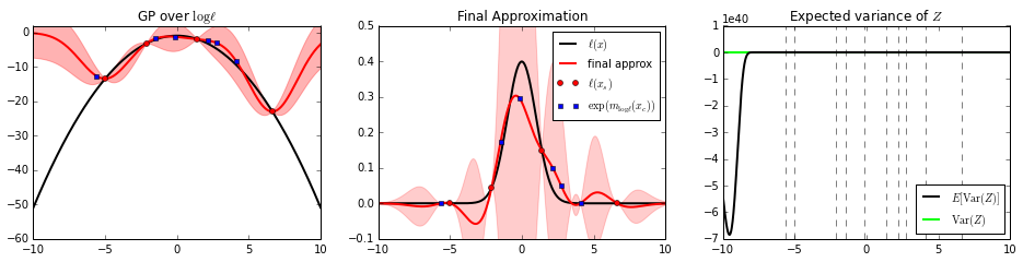
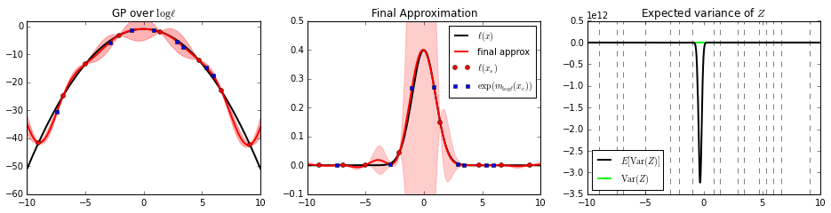
add(bq)

x = 1.4052910677
E[Z] = 1.81816144454e-05
V(Z) = 4.95413041126e-09
Z = 0.0000 [-0.0001, 0.0002]

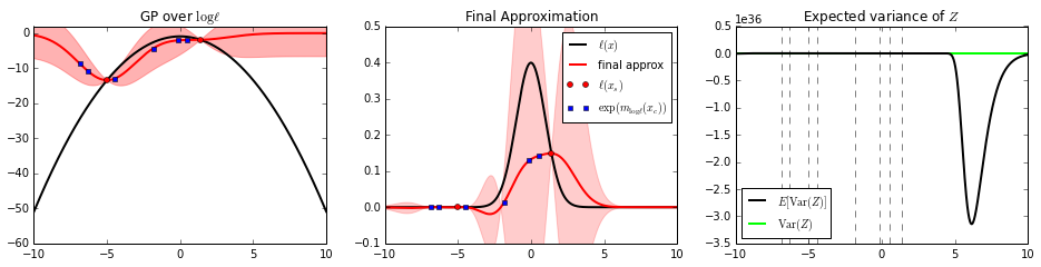
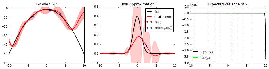
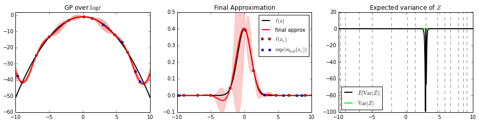
add(bq)

x = 6.64358430235
E[Z] = 0.0655204987334
V(Z) = 0.0126525192528
Z = 0.0655 [-0.1549, 0.2860]

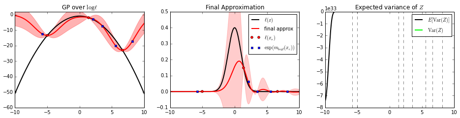
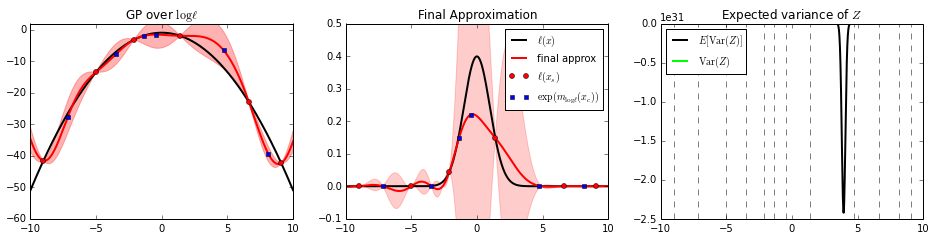
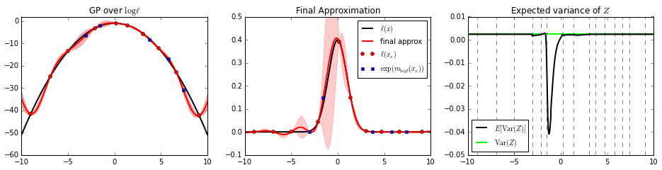
add(bq)

x = -2.09951783218
E[Z] = 0.0586980981797
V(Z) = 0.0207373317676
Z = 0.0587 [-0.2236, 0.3409]

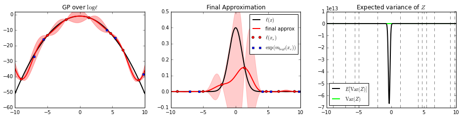
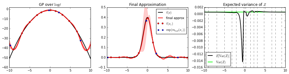
add(bq)

x = -9.01101433922
E[Z] = 0.103667506169
V(Z) = 0.0763855441687
Z = 0.1037 [-0.4380, 0.6454]

add(bq)

x = 9.1002318972
E[Z] = 0.0752797700545
V(Z) = 0.0203972059936
Z = 0.0753 [-0.2046, 0.3552]

add(bq)

x = 4.71861182049
E[Z] = 0.0931528467188
V(Z) = 0.0373985303269
Z = 0.0932 [-0.2859, 0.4722]

add(bq)

x = -6.90978217015
E[Z] = 0.0610104395892
V(Z) = 0.0053876473346
Z = 0.0610 [-0.0829, 0.2049]

add(bq)

x = 0.196855581753
E[Z] = 0.124567153682
V(Z) = 0.120224063159
Z = 0.1246 [-0.5550, 0.8042]

add(bq)

x = 3.08558498792
E[Z] = 0.121650895453
V(Z) = 0.00415513324733
Z = 0.1217 [-0.0047, 0.2480]

add(bq)

x = -3.20225408927
E[Z] = 0.126989779828
V(Z) = 0.00235994553969
Z = 0.1270 [0.0318, 0.2222]

add(bq)

x = -1.00877980771
E[Z] = 0.117121406149
V(Z) = 0.000535153011259
Z = 0.1171 [0.0718, 0.1625]

add(bq)

x = 7.5969086774
E[Z] = 0.119578413594
V(Z) = 9.60697466024e-08
Z = 0.1196 [0.1190, 0.1202]